Friday, June 16, 2017

Subsurface Scattering

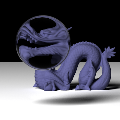
I chose to implement subsurface scattering for the term project of the course. My first intention was to implement one of the diffusion approximation algorithms. Although they are much more faster than simulating transfer of equation with volumetric path tracing, they either do not work with arbitrary geometry or need a preprocessing step which I found cumbersome. Therefore, I implemented a volumetric path tracer that simulates subsurface scattering. The most challenging part for me was to find appropriate absorption and scattering coefficients for the tests. Thankfully, series of outputs show the effect of the scattering inside the medium clearly. Also, I captured a video to show the progressive feature of my path tracer.

Additionaly, I changed the scene input format quite a bit. I used assimp to load the 3d models. Since it supports many of the popular extensions, scene design is much more flexible than before. An example scene file is here.

Here are the outputs for the same scene with different material settings that my path tracer supports.
Lambertian Material
kd: (1.0, 1.0, 1.0)
2109 samples
Perfect Specular Material
ks: (1.0, 1.0, 1.0)
1785 samples
Perfect Refractive Material
tintcolor: (0.79, 0.53, 0.79)
tintdistance: 0.2
index of refraction: 2.0
2470 samples
Translucent Material
tintcolor: (0.79, 0.53, 0.79)
tintdistance: 0.2
index of refraction: 2.0
scattering coefficient: 50
anisotropy: 0.7
1015 samples
Translucent Material
tintcolor: (0.0, 0.8, 0.0)
tintdistance: 0.1
index of refraction: 1.5
scattering coefficient: 100
anisotropy: 0.7
3311 samples
Translucent Material
tintcolor: (0.8, 0.8, 0.8)
tintdistance: 0.2
index of refraction: 1.0
scattering coefficient: 150
anisotropy: 0.7
4900 samples
Finally, here is a video to demonstrate the progressive feature.

Monday, June 5, 2017

Assignment 9: Monte Carlo Path Tracing

We have not considered any radiance contribution coming from the indirect sources to the surface of interactions. The model we have used so far couldn't simulate the global illumination and we had to fake it by adding an ambient term. Even if the ambient term can be adjusted to a reasonable level, we cannot simulate phenomena, such as color bleeding, caustics, etc., that can only be simulated correctly by global illumination algorithms. Therefore, it is a must to implement a global illumination algorithm to produce more realistic images.

In this assignment, we are required to solve the rendering equation by using monte carlo techniques. Producing an unbiased image with a low variance is not a simple task and has been a research topic since the early days of this field. Thankfully, there are great resources offering several variance reduction techniques to reduce the noise and for faster convergence. Here are some of the resources I have been using:

After reading and learning a lot from these resources, I started to implement my path tracer. Although my path tracer is very simple and using a few of the techniques that I've learned, I am planning to implement them in time. For now, my path tracer has the following features:
  • Progressive path tracing: It is great to see your images converge in real-time and to move around the scene you created. For most of the scenes, I take interactive frame rates.
  • Cosine weighted importance sampling: It is the only variance reduction strategy I used for the indirect lighting calculation. However, in future, an importance sampling for the bsdf term seems inevitable.
  • Explicit light sampling: At every bounce, I take samples from each light source. If many light sources are involved, we may choose one of them uniformly or by a pdf that we defined according to some criteria, for example, power of lights.
  • Smooth dielectrics: Perfectly reflective and refractive surfaces are easy to implement if you already implemented them in your ray tracer. Since they have delta distributions, only a single path is meaningful to follow. Therefore, everything is the same as in the case of our old ray tracer. However, we do not send both reflected and refracted rays for our refractive surfaces since the recursion would be an overhead in general and it is already deadly for the performance of the CUDA programs. Instead, we choose one of them with probability determined by the fresnel equations, which I talked about in the previous posts. 

Also, I am planning to
  • read this paper to implement both refraction and reflection for the rough surfaces.
  • add multiple importance sampling for direct lighting to reduce the noise related to glossy reflections.
  • add importance sampling for the bsdf term of the indirect lighting.

Finally, let me sum the basic things up for a path tracer in some brief paragraphs. We separate incoming radiance sources into two parts as direct and indirect. We sample lights explicitly for the direct part and while sampling this part, it is reasonable to importance sample the lights as well as BSDFs. For the indirect part, however, we have no idea about which direction may potentially give us higher radiance values since it is the problem itself that we want to solve. However, we can say which direction can contribute more according to the cosine term and BSDF.

Furthermore, since we explicitly sample the lights, if we hit any area light source with the indirect rays we have sent, we cannot take any contributions from the light sources we already sampled in the previous bounce. That is, if we hit a light that we already sampled, we consider as if it does not contribute. Also, beware that we do not sample the lights explicitly for perfectly reflective and refractive surfaces because that would be meaningless due to their delta distributions. Therefore, if the rays that have been sent after the interaction with smooth surfaces hit a light source, we take the contribution coming from these rays.

As before, I used jittered samples to send the rays not only to the center of the pixels but to the entire square owned by the pixel.

I tried several russian roulette strategies and fixed depth values for ray terminations. While russian roulette can make a substantial decrease in fps, fixed depth values result in better performance. However, unlike fixed depth values, russian roulette generates unbiased images, which is more important for me now. The outputs shown below are generated using russian roulette that considers the radiance contribution weight of the ray.

Let us see the outputs.
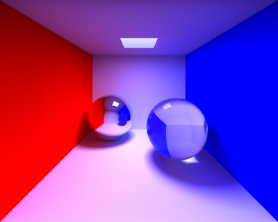
Cornellbox rendered with 3800 samples
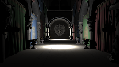
Sponza considering only direct illumination
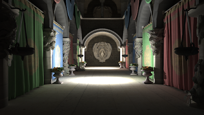
Sponza rendered with 650 samples.
Color Bleeding Effect
Caustic Effect
Nothing Special

Sunday, May 14, 2017

Assignment 8: BRDF Models

I have used well-known Blinn–Phong shading model so far in my project. However, it is not physically accurate since it does not consider normalization factor. Also, if we do not use the modifed version of Blinn–Phong shading model, we may not properly normalize it. Therefore, to get more realistic results, one may use the modifed version with normalization factor. The same applies for the Phong shading model.

On the other hand, we are required to implement a physically based BRDF model, Cook-Torrance. It simulates specular reflection by treating every surface as if they consist of many microfacets. In this model, we consider fresnel reflectance of the surface, distribution of microfacets by using a distribution function and the geometrical outcomes, blocking and masking, of this distribution.

Let us see the images of this week.
output of brdf_phong_original.xml
kernel execution time: 6.1 milliseconds
output of brdf_phong_modified.xml
kernel execution time: 6.1 milliseconds
output of brdf_phong_modified_normalized.xml
kernel execution time: 6.1 milliseconds
output of brdf_blinnphong_original.xml
kernel execution time: 6.1 milliseconds
output of brdf_blinnphong_modified.xml
kernel execution time: 6.1 milliseconds
output of brdf_blinnphong_modified_normalized.xml
kernel execution time: 6.1 milliseconds
output of brdf_torrancesparrow.xml
kernel execution time: 6.1 milliseconds
output of killeroo_blinnphong_modified_normalized.xml
kernel execution time: 57 milliseconds
output of killeroo_blinnphong_modified_normalized.xml
kernel execution time: 63 milliseconds
output of killeroo_torrancesparrow.xml
kernel execution time: 57 milliseconds
output of killeroo_torrancesparrow.xml
kernel execution time: 63 milliseconds

Sunday, April 30, 2017

Assignment 6&7: Texture Mapping, Procedural Textures and Bump Mapping

Textures add an important portion of realism to ray tracers. Using just plain colors is not enough to create real world scenes and this is why it is almost a must for every ray tracer.

For these two assigments, I implemented texture mapping, perlin noise textures and bump mapping. CUDA helped me, it does once in a while, for texture operations such as fetching, filtering and setting up many sampling parameters. Figuring out which function to use and how to use it was a bit painful but now all is clear and I will talk about them in the "Lessons learned" section. Also, I implemented the improved perlin noise to produce procedural textures.

Bump mapping is relatively easy when you add the texturing functionality to your ray tracer. However, there is one big problem when dealing with the tangent vectors and the surface normal. How are you going to transform them if you are using instancing? Transforming the normal is well-known but what about others? Of course, we will not transform the tangent vectors in the way we transform the normals. Say, you figured out that you should use the transformation matrix M but not the inverse-transpose of M. However, it will work unless you have a transformation matrix whose determinant is negative. If your transformation matrix has a negative determinant then everything changes. Thanks to one of my friend who gave me this information, I was able to solve the problem by taking tangent vectors from object space to world space by transforming them with M and after that by multiplying one of the tangent vectors by the sign of the determinant of M.

Let us see the outputs of this week.
output of simple_texture.xml
kernel execution time: 9.7 milliseconds
output of the skybox.xml
kernel execution time: 923 milliseconds
output of ellipsoids_texture.xml
kernel execution time: 11.4 milliseconds
output of sphere_texture_blend_bilinear.xml
kernel execution time: 10.7 milliseconds
output of sphere_texture_replace_nearest.xml
kernel execution time: 10.8 milliseconds
output of sphere_texture_replace_bilinear.xml
kernel execution time: 10.9 milliseconds
output of killeroo_diffuse_specular_texture.xml
kernel execution time: 492 milliseconds
output of perlin_types.xml
kernel execution time: 14.1 milliseconds
output of bump_mapping_basic.xml
kernel execution time: 350 milliseconds
output of bump_mapping_transformed.xml
kernel execution time: 335 milliseconds
output of killeroo_bump_walls.xml
kernel execution time: 515 milliseconds
output of sphere_bump_nobump.xml
kernel execution time: 192 milliseconds
Lessons learned:
  1. I stored the random number sequence for the perlin noise in the constant memory. Since the numbers are constant during the execution, constant memory is the fast and appropriate solution.
  2. Texturing with CUDA is really simple. The only confusing part is to use which function and how. First of all, I recommend you to implement a texture manager class which manages all the textures loaded for your scene. Your scene file may use the same texture more than once and you might create space for the same image for many times. Following code snippet summarizes how to create a texture in CUDA.
       
cudaArray* cuda_array = nullptr;

//1-Create and fill a channel description.
cudaChannelFormatDesc channel_desc = cudaCreateChannelDesc(8, 8, 8, 8, cudaChannelFormatKindUnsigned); //RGBA

HANDLE_ERROR(cudaMallocArray(&cuda_array, &channel_desc, image_width, image_height));
HANDLE_ERROR(cudaMemcpyToArray(cuda_array, 0, 0, bits, //"bits" is the pointer to your image on the host memory
             image_width * image_height * 4, cudaMemcpyHostToDevice)); 
        
//2-Create and fill a resource description.
cudaResourceDesc res_desc;
memset(&res_desc, 0, sizeof(res_desc));
res_desc.resType = cudaResourceTypeArray;
res_desc.res.array.array = cuda_array;

//3-Create and fill a texture description.
cudaTextureDesc tex_desc;
memset(&tex_desc, 0, sizeof(tex_desc));
tex_desc.addressMode[0] = cudaAddressModeClamp;
tex_desc.addressMode[1] = cudaAddressModeClamp;
tex_desc.filterMode = cudaFilterModeLinear;
tex_desc.readMode = cudaReadModeNormalizedFloat;
tex_desc.normalizedCoords = 1;

//4-Create the texture object
cudaTextureObject_t texture = 0;
HANDLE_ERROR(cudaCreateTextureObject(&texture, &res_desc, &tex_desc, nullptr));

..
..
..
..


//Fetch a pixel.
float4 pixel = tex2D<float4>(texture , u, v);
Beware that we do not bind any texture before using it since we are using texture objects but not texture references. To understand the difference and which parameter does what, you should see the documentation.

Tuesday, April 18, 2017

Assignment 5: Distributed Ray Tracing

Although we have rendered some nice pictures so far, we didn't concentrate on making them more realistic. By looking at them closely, we can easily see hard shadows and jaggy edges which are the fundamental problem of computer generated images. In this assignment, we concentrate more on this so that we can have softer shadows and less jaggy edges by means of multisampling. Of course there are ways to post-process the final images to have more realistic ones but that would be another topic of discussion. Unfortunately, realism comes at a price in our case, regardless to say it is worth it, since we are now sending more and more rays for a pixel.

Taking more than one sample per pixel does not only help to implement multisampling but it also makes it possible to have area lights, depth of field and some other nice things without a further cost. Our starting point is to choose some random points around a pixel center and consider all the radiance values computed for the rays shot from these points when calculating the final value of this particular pixel. Many strategies can be adopted for choosing these random points and combining radiance values we get. Easiest one is to select all the points just randomly. However, "just randomly" creates quite noisy images. Instead of this, we can adopt jittered sampling, multi-jittered sampling, n-rooks sampling and many more. I implemented jittered sampling and the results are quite satisfying. For the "combining" part, I basically take the average of the radiance values resulted from these rays.

Once you calculated the jittered sample for a pixel, you can use this sample for the area light and the depth of field part as well. For example, say you are going to take 36 samples for your scene. That means you will take 36 jittered sample points around the pixel, 36 different sample points on the area light and 36 different sample points on the aperture of the thin lens camera. Once you take one of this sample, you can use it for the others too. This way, you will have more uniformly distributed samples on each of the planes you are sampling. Of course, this may not apply if you want to take more samples for area lights but not for multisampling or for other combinations that you might want different number of samples.

Ray Tracing from the Ground Up explains these concepts clearly. Also, you can see this to pick a random point on a disk, which you are going to need for disk shaped area lights and for depth of field effect.

Apart from these subjects, I implemented what I've explained in the "lessons learned" part of the previous post. I reduced the rendering time from 1.34 seconds to 0.47 seconds for the image below.
previous approach, 32 samples
mentioned approach, 169 samples
mentioned approach, 32 samples


However, not unexpectedly, the resulting images are a bit noisy. Considering that we are going to take more and more samples when we deal with Monte Carlo method, this approach will be the right choice for sure.

Lastly, let us see what we rendered this week.
output of glass_plates_point.xml
kernel execution time: 1.34 seconds
output of glass_plates_area.xml
kernel execution time: 1.37 seconds
output of dragon_spot_light.xml
kernel execution time: 26.7 milliseconds
output of dragon_spot_light_msaa.xml
kernel execution time: 2.07 seconds
output of spheres_dof.xml
kernel execution time: 331 milliseconds
output of metal_plates_area.xml
kernel execution time: 1.07 seconds
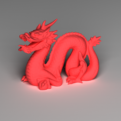
The dragon under an area light

Sunday, April 9, 2017

Assignment 4: Reflections and Refractions

Ray tracing is good at simulating refraction and reflection of light by its nature. One of the first things we have to consider to simulate reflective and refractive materials is that we have to shoot rays beside the primary and shadow rays. After primary rays, if we detect any refractive or reflective surface, we should generate new rays based on the physics of light.

A perfect specular surface reflects the incoming light in a certain direction. Although perfect specular surfaces are hard to find in nature, not sure if it is impossible, they are implemented in every ray tracer since they are the starting point for simulating other reflective surfaces. On the other hand, when the light interacts with a refractive surface, some of the photons are reflected while some others are refracted depending on the incident angle of light. This effect can be easily seen from the picture of a lake below.
As you can see, in the pixels near the right-bottom corner of the image, we can easily see the transparent nature of water. The reason is that the incident angle is smaller. However, as the view direction is getting to be perpendicular to the surface normal, incident angle is getting larger and therefore photons are getting mostly reflected. Fresnel equations explain this behaviour and based on these equations, we can compute which proportion of photons will be reflected or refracted. Furthermore, Schlick’s approximation is a well-known approximation of the Fresnel equations, which can be used to decrease the computation time. Also, Snell's law helps us to compute the direction of a refracted light. Finally, by means of the Beer's law, we can compute the attenuation of the light traveling through the medium. This document clearly explains aforementioned equations and laws except Beer's law.

Let us see the scenes we should render for this assignment.
output of cornellbox_glass.xml
kernel execution time: 31.1 milliseconds

output of horse_and_glass_mug.xml
kernel execution time: 571 milliseconds

output of glass_plates.xml
kernel execution time: 55.8 milliseconds

output of killeroo_glass.xml
kernel execution time: 531 milliseconds

output of killeroo_half_mirror.xml
kernel execution time: 82.5 milliseconds

output of killeroo_mirror.xml
kernel execution time: 82.5 milliseconds
Lessons learned:
  1. Rendering times are higly increased for the scenes which include refractive materials. Of course this is an expected outcome, however, the biggest reason for slowdown is the usage of stack which is used to recursively trace all the rays generated by these materials. Even without recursion, that is, just defining a stack of 2 kb in every thread and not touching it, my ray tracer slows down by 2x. A workaround to this problem is as follows: instead of generating two rays after light-refractive surface interaction, we generate one ray but we choose whether to refract or reflect the ray by means of Fresnel equations or Schlick's approximation and a uniform random number generator. The problem is that if we take just one sample for each pixel, the output might look incorrect. Therefore, we should take as many samples as possible for each pixel since the output converges to the expected output with infinitely many samples. For these reasons, I postponed the implementation of this approach to the next assignment where I will implement multisampling. After implementing this approach, every ray-surface interaction will be able to generate at most one ray so that I get rid of the stack.